Props Cannot Be Imported Again Nureal
The Complete Guide to Neural Network multi-class Nomenclature from scratch
What on world are neural networks? This article volition requite yous a full and complete introduction to writing neural networks from scratch and using them for multinomial classification. Includes the python source code.
Neural networks reflect the beliefs of the human being brain. They allow programs to recognise patterns and solve common problems in machine learning. This is another option to either perform classification instead of logistics regression. At Rapidtrade, we use neural networks to classify data and run regression scenarios. The source code for this article is available on GitHub.
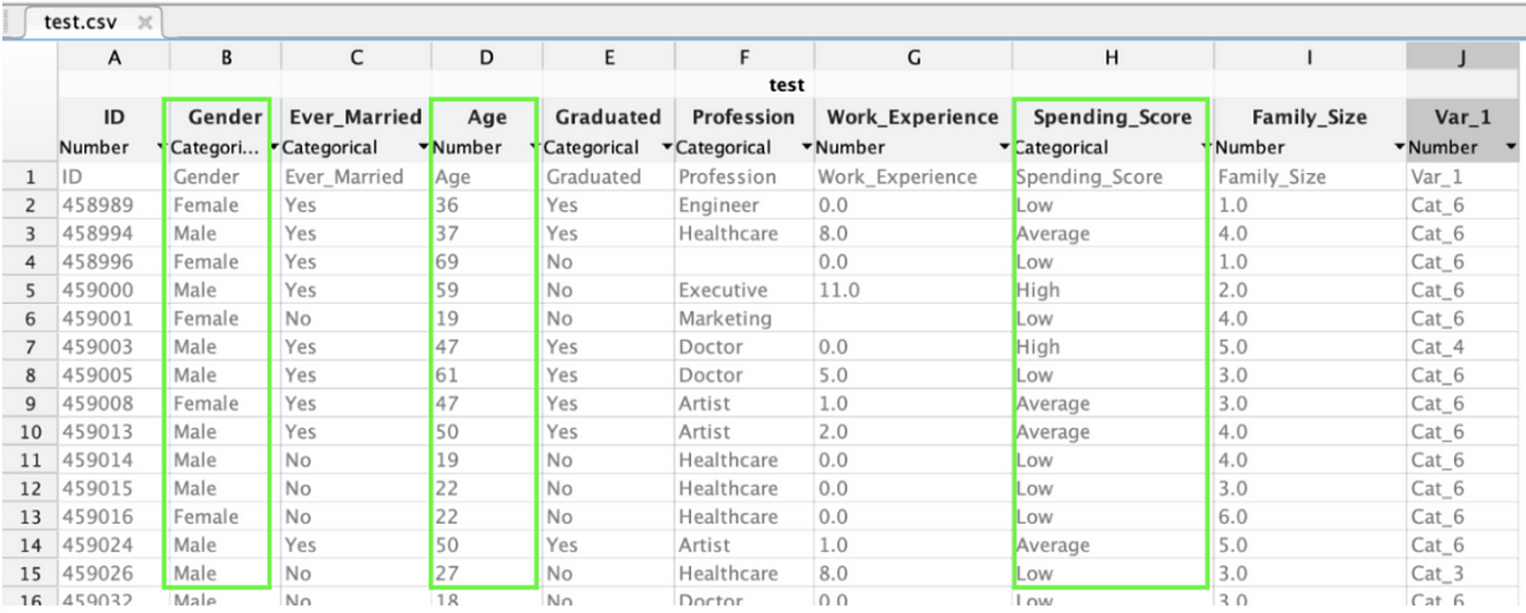
We will exist working with a dataset from Kaggle and you can download it hither. So to visualise the data we will be working with in this article, encounter below. Nosotros will employ this to train the network to categorise our customers co-ordinate to column J. Nosotros will also utilise the 3 features highlighted to classify our customers.
I needed 3 features to fit my neural network and these were the best 3 bachelor.
Just go on in heed, nosotros will convert all the alpha cord values to numerics. After all, we can't plug strings into equations ;-)
This is quite a long article and is broken up into 2 sections:
- Introduction
- Putting it all together
Skillful luck ;-)
Introduction
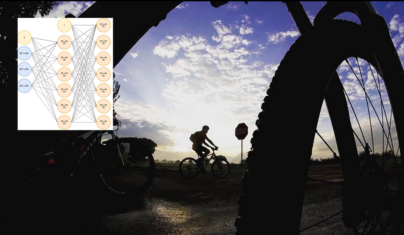
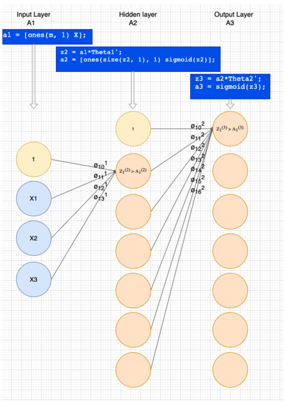
Neural networks are always made up of layers, as seen in figure two. It all looks complicated, but let's unpack this to make it more understandable.
A neural network has 6 important concepts, which I will explain briefly here, just cover in particular in this series of articles.
- Weights — These are similar the theta's we would use in other algorithms
- Layers — Our network will take 3 layers
- Forward propagation — Use the features/weights to become Z and A
- Back propagation — Employ the results of forward propogation/weights to get S
- Calculating the cost/gradient of each weight
- Gradient descent — find the best weight/hypothesis
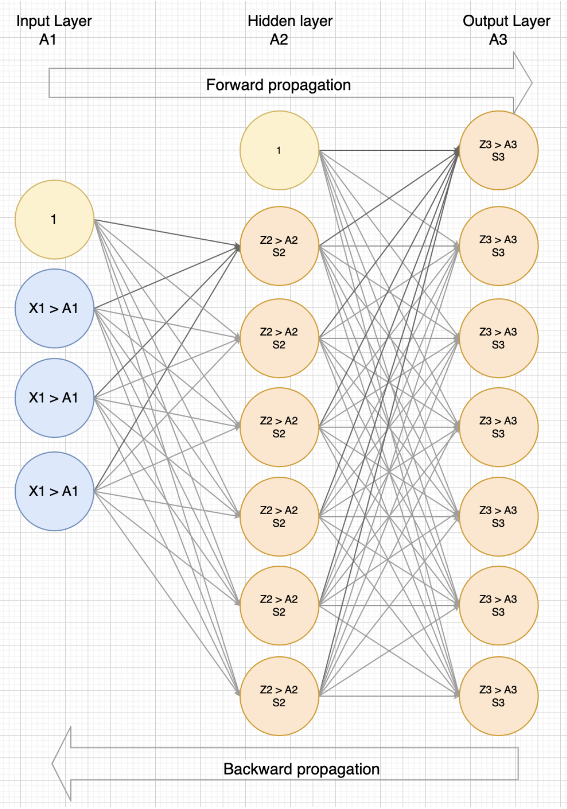
In this series, we volition be building a neural network with 3 layers. Let's discuss these layers quickly before nosotros get into the tick of it.
- Input Layer
Refer to figure 2 higher up and nosotros will refer to the result of this layer every bit A1. The size (# units) of this layer depends on the number of features in our dataset.
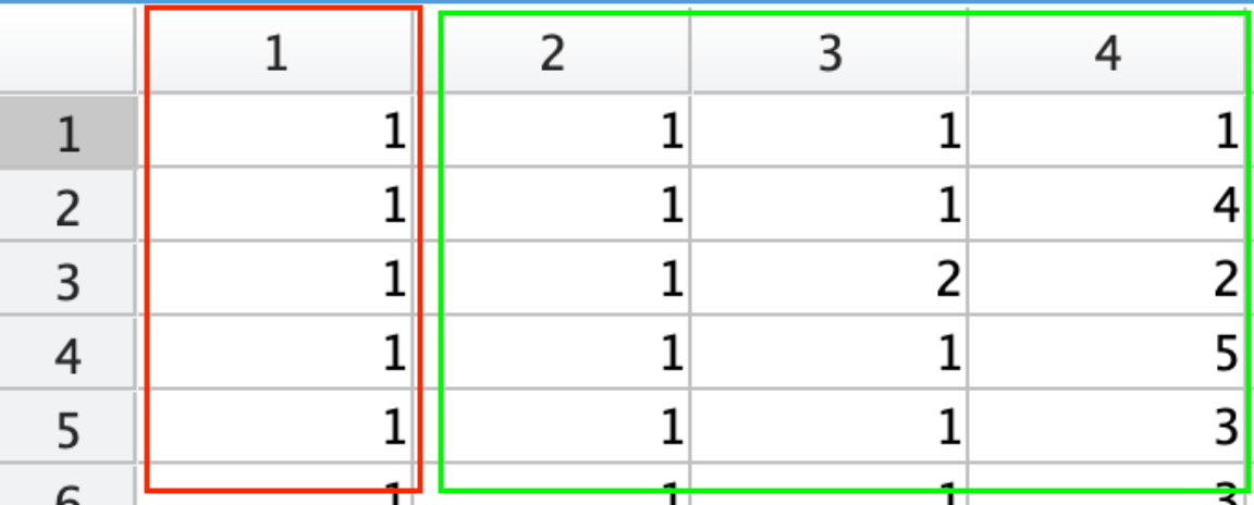
Building our input layer is not difficult you just re-create X into A1, simply add what is called a biased layer, which defaults to "1".
Col 1: Biased layer defaults to 'ane'
Col 2: "Ever married" our 1st feature and has been re-labeled to i/2
Col 3: "Graduated" our second feature and re-labeled to 1/2
Col iv: "Family size" our 3rd feature
- Hidden layer
Refer to figure 2 to a higher place and nosotros only have ane hidden layer, but you could accept a subconscious layer per feature. If you had more hidden layers than the logic I mention below, you would replicate the calculations for each hidden layer.
The size (#units) is upwardly to y'all, nosotros accept chosen #features * 2 ie. 6 units.
This layer is calculated during forward and astern propagation. After running both these steps, we calculate Z2, A2 and S2 for each unit. See below for the outputs once each of these steps is run.
Forward propagation
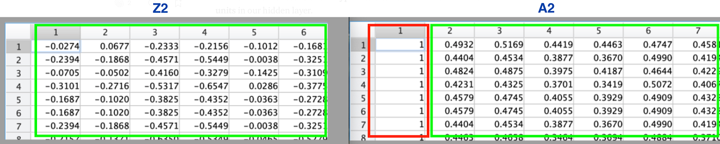
Refer to figure 1 equally in this step, we summate Z2 so A2.
- Z2 contains the results of our hypothesis calculation for each of the half dozen units in our hidden layer.
- While A2 as well includes the biased layer (col 1) and has the sigmoid function practical to each of the cell'due south from Z2.
Hence Z2 has 6 columns and A2 has 7 columns every bit per figure 4.
Back propagation
So, afterward forwards propagation has run through all the layers, we then perform the back propagation step to summate S2. S2 is referred to equally the delta of each units hypothesis calculation. This is used to and so figure out the gradient for that theta and afterward, combining this with the cost of this unit, helps gradient descent figure out what is the best theta/weight.
- Output layer
Our output layer gives united states the result of our hypothesis. ie. if these thetas were applied, what would our best guess be in classifying these customers. The size (#units) is derived from the number labels for Y. As can become seen in figure ane, at that place are 7 labels, thus the size of the output layer is vii.
Every bit with the hidden layer, this result is calculated during the two steps of forward and backward propagation. After running both these steps, here is the results:
Forward propagation
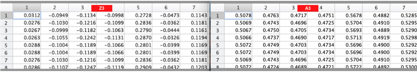
During frontwards prop, nosotros volition summate Z3 and A3 for the output layer, as we did for the subconscious layer. Refer to figure i above to see there is no bias column needed and yous tin see the results of Z3 and A3 below.
Back propagation
Now that (referring to figure one) nosotros take Z3 and A3, lets summate S3. As it turns out S3 is only a basic cost calculation, subtracting A3 from Y, so we will explore the equations in the upcoming articles, merely we can nonetheless see the upshot beneath
Putting it all together
So, the to a higher place is a piffling bad-mannered as it visualises the outputs in each layer. Our chief focus in neural networks, is a office to compute the cost of our neural network. The coding for this function will take the following steps.
- Prepare the data
- Setup neural network
- Initialise a set of weights/thetas
- Create our price part which volition
iv.ane Perform forwards propagation
4.two Calculate the cost of forrard propagation
four.iii Perform astern propagation
4.4 Calculate the deltas then gradients from backward prop. - Perform cost optimisation
5.i Validates our cost part
five.2 That performs gradient descent on steps (four.ane) to (iv.4) until it finds the best weight/theta to use for predictions - Predict results to check accuracy
1. Prepare the data
To begin this exploratory analysis, get-go import libraries and define functions for plotting the data using matplotlib. Depending on the data, not all plots will be made.
Hey, I'm only a simple kerneling bot, non a Kaggle Competitions Grandmaster!
          from mpl_toolkits.mplot3d import Axes3D
from sklearn.preprocessing import StandardScaler
from sklearn.preprocessing import LabelEncoder
import seaborn as sns
import matplotlib.pyplot as plt # plotting
import numpy every bit np # linear algebra
import os # accessing directory structure
import pandas as pd # data processing, CSV file I/O (eastward.g.
from scipy import optimize as opt          pd.read_csv)
import matplotlib.pyplot equally plt
Now, let'southward read our data and have a quick wait.
          df = pd.read_csv('customertrain.csv')
df.head() 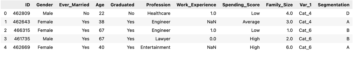
Doing an info, we can see we have some work to exercise with goose egg values equally well as some object fields to catechumen to numerics.
df.info() 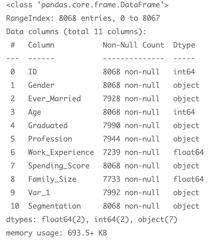
So, let's transform our object fields to numerics and drib the columns we practise non need.
          columns = ["Gender","Ever_Married","Graduated","Profession","Spending_Score"]
for feature in columns:
            le = LabelEncoder()
            df[feature] = le.fit_transform(df[characteristic])          df = df.drop(["ID","Gender","Age","Profession","Work_Experience","Spending_Score"], axis=ane)
df.dropna(subset=['Var_1'], inplace=True)          df.caput()
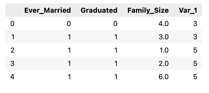
Utilise fit_transform to encode our multinomial categories into numbers we can piece of work with.
          yle = LabelEncoder()
df["Var_1"] = yle.fit_transform(df["Var_1"])
df.head()
Make full in missing features
An important office of regression is understanding which features are missing. We tin can choose to ignore all rows with missing values, or fill them in with either manner, median or fashion.
- Mode = about common value
- Median = center value
- Mean = boilerplate
Hither is a handy function you can call which volition fill in the missing features past your desired method. Nosotros volition choose to fill up in values with the boilerplate.
After funning below, you lot should see 7992 with no nothing values.
          def fillmissing(df, characteristic, method):
            if method == "mode":
            df[characteristic] = df[feature].fillna(df[feature].mode()[0])
            elif method == "median":
            df[feature] = df[feature].fillna(df[feature].median())
            else:
            df[characteristic] = df[feature].fillna(df[feature].mean())
features_missing= df.columns[df.isna().any()]
for feature in features_missing
            fillmissing(df, feature= characteristic, method= "hateful")          df.info()
Extract Y
Let's excerpt our Y column into a separate array and remove it from the dataframe.
Y = df["Var_1"] df = df.drop(["Var_1"], axis=1
Now copy out our X and y columns into matrices for easier matrix manipulation later.
          X = df.to_numpy() # np.matrix(df.to_numpy())
y = Y.to_numpy().transpose() # np.matrix(Y.to_numpy()).transpose()
m,due north = X.shape
Normalize features
At present, allow's normalise X and so the values prevarication between -i and 1. We do this so nosotros tin can go all features into a similar range. We use the post-obit equation

The goal to perform standardization is to bring down all the features to a common scale without distorting the differences in the range of the values. This process of rescaling the features is so that they have hateful as 0 and variance every bit 1.
2. Setup neural network
Now, we tin setup the sizes of our neural network, first, below is the neural network we want to put together.
Below initialisations, ensure above network is accomplished. So, now you are asking "What are reasonable numbers to prepare these to?"
- Input layer = set up to the size of the dimensions
- Subconscious layers = ready to input_layer * two
- Output layer = set to the size of the labels of Y. In our case, this is seven categories
          input_layer_size = northward                      # Dimension of features
hidden_layer_size = input_layer_size*two    # of units in hidden layer
output_layer_size = len(yle.classes_)     # number of labels
iii. Initialise weights (thetas)
Equally it turns out, this is quite an important topic for slope descent. If y'all have not dealt with gradient descent, then check this article first. We tin can meet above that we need 2 sets of weights. (signified by ø).
Nosotros oftentimes still calls these weights theta and they mean the same thing.
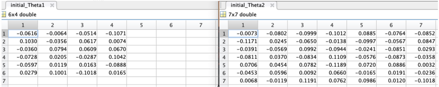
We need 1 set up of thetas for level ii and a 2nd set for level three. Each theta is a matrix and is size(L) * size(L-1). Thus for above:
- Theta1 = 6x4 matrix
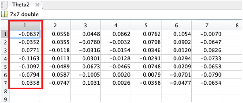
- Theta2 = 7x7 matrix
Nosotros take to now approximate at which initial thetas should be our starting point. Here, epsilon comes to the rescue and below is the matlab code to easily generate some random pocket-sized numbers for our initial weights.
          def initializeWeights(L_in, L_out):
            epsilon_init = 0.12
            W = np.random.rand(L_out, 1 + L_in) * 2 * \
            epsilon_init - epsilon_init
            return W
After running above office with our sizes for each theta as mentioned to a higher place, nosotros will become some good pocket-sized random initial values equally in figure vii. For effigy 1 above, the weights we mention would refer to rows 1 in beneath matrix's.
four. The cost function
We need a function which can implement the neural network cost part for a two layer neural network which performs classification.
In the GitHub lawmaking, checknn.py our costfunction called nnCostFunction will return:
- gradient should be a "unrolled" vector of the partial derivatives of the neural network
- the final J which is the cost of this weight.
Our cost function will need to perform the following:
- Reshape nn_params back into the parameters Theta1 and Theta2, the weight matrices for our 2 layer neural network
- Perform frontwards propagation to calculate (a) and (z)
- Perform backward propagation to utilize (a) calculate (southward)
So, our cost function kickoff upwards, needs to reshape our thetas back into a theta for the subconscious and output layers.
          # Reshape nn_params back into the parameters Theta1 and Theta2,
# the weight matrices for our 2 layer neural network          Theta1 = nn_params[:hidden_layer_size * \
            (input_layer_size + i)].reshape( \
            (hidden_layer_size, input_layer_size + one))
Theta2 = nn_params[hidden_layer_size * \
            (input_layer_size + 1):].reshape( \
            (num_labels, hidden_layer_size + 1))          # Setup some useful variables
yard = Ten.shape[0]
4.ane Frontward propagation
Forrard propagation is an important part of neural networks. Its not as difficult as it sounds.
In effigy 7, we tin come across our network diagram with much of the details removed. We will focus on ane unit of measurement in level ii and one unit of measurement in level iii. This agreement tin then exist copied to all units. Take note of the matrix multiplication we can do (in blueish in effigy 7) to perform forward propagation.
I am showing the details for one unit of measurement in each layer, but you can repeat the logic for all layers.
Before we evidence the forward prop code, lets talk a little on the 2 concepts we need during forward prop.
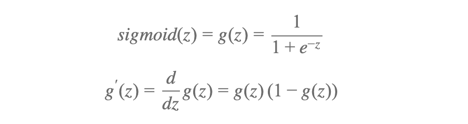
iv.1.1 Sigmoid functions
Since we are doing nomenclature, we will use sigmoid to evaluate our predictions. A sigmoid office is a mathematical office having a characteristic "Due south"-shaped curve or sigmoid bend. A common case of a sigmoid function is the logistic office shown in the offset figure and defined by the formula
In github, in checknn.py the following handy functions are created:
- sigmoid is a handy role to compute sigmoid of input parameter Z
- sigmoidGradient computes the gradient of the sigmoid function evaluated at z. This should work regardless if z is a matrix or a vector.
          def sigmoid(z):
            m = np.frompyfunc(lambda x: 1 / (1 + np.exp(-x)), one, i)
            render thousand(z).astype(z.dtype)          def sigmoidGradient(z)
            return sigmoid(z) * (1 - sigmoid(z))
4.1.two Regularization
We will implement regularization as one of the most common problems information scientific discipline professionals face is to avoid overfitting. Overfitting gives yous a situation where your model performed exceptionally well on train data just was not able to predict test data. Neural network are circuitous and makes them more decumbent to overfitting. Regularization is a technique which makes slight modifications to the learning algorithm such that the model generalizes better. This in turn improves the model's performance on the unseen data as well.
If you lot have studied the concept of regularization in machine learning, you lot will have a fair idea that regularization penalizes the coefficients. In deep learning, it really penalizes the weight matrices of the nodes.
We implement regularization in nnCostFunction by passing in a lambda which us used to penalise both the gradients and costs that are calculated.
4.1.iii Implementing forward prop
Every bit per effigy one, lets calculate A1. Yous tin can encounter that its pretty much my Ten features an nosotros add the bias cavalcade hard coded to "1" in front. Here is the python lawmaking to practice this:
          # Add together ones to the Ten data matrix
a1 = np.insert(Ten, 0, 1, axis=1)
The result will now give you the results in A1 in effigy iv. Take special notation of the bias column "ane" added on the front.
Great, thats A1 washed, lets move onto A2. Before nosotros get A2, we will commencement run a hypothesis to summate Z2. In one case you have the hypotheses, you can run it through the sigmoid function to go A2. Again, as per effigy 1, add together the bias column to the front.
          # Perform forward propagation for layer 2
z2 = np.matmul(a1, Theta1.transpose())
a2 = sigmoid(z2)
a2 = np.insert(a2, 0, 1, axis=1)
Ok, so we almost there…. Now onto A3, lets do the same as with A2, simply this time, we dont worry to add together the bias column.
          z3 = np.matmul(a2, Theta2.transpose())
a3 = sigmoid(z3)
You lot may exist request, "why do we keep Z2 & Z3". Well, we volition need those in back propagation. So we may as well keep them handy ;-).
4.two Summate the cost of forward prop
Earlier we continue, if you empathize our Y column (figure ix) which contains the labels used to categorise our customers. So to calculate the cost we need to reformat Y into a matrix which corresponds to the number of labels. In our case we accept 7 categories for our customers.
Effigy 8, shows how Y is converted to a matrix y_one_hot and labels are now indicated as a binary in the appropriate cavalcade.
          # plow Y into a matrix with a new column for each category and marked with ane
y_one_hot = np.zeros_like(a3)
for i in range(thousand):
y_one_hot[i, y[i] - ane] = 1 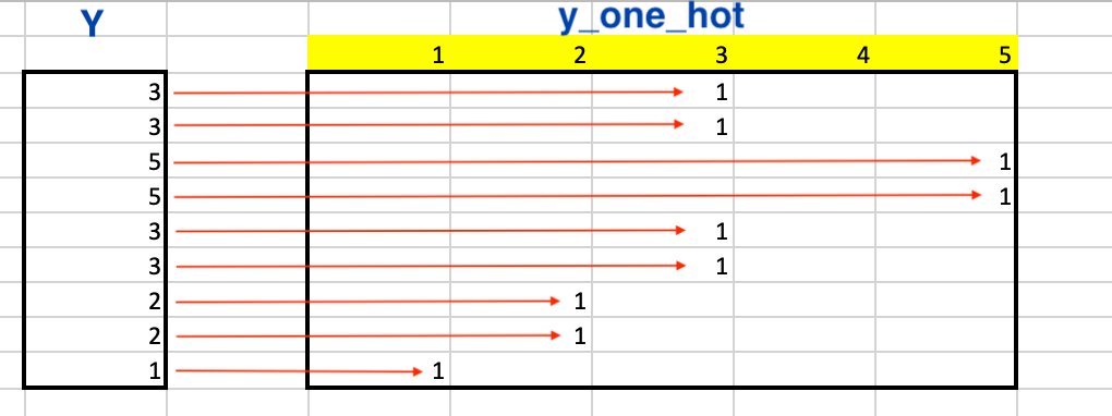
Now that we accept Y in a matrix format, lets take a look at the equation to calculate the price.

Well, that's all very complicated, but good news is that with some matrix manipulation, we can practice it in a few lines of python code as below.
          # Calculate the cost of our forrard prop
ones = np.ones_like(a3
A = np.matmul(y_one_hot.transpose(), np.log(a3)) + \
            np.matmul((ones - y_one_hot).transpose(), np.log(ones - a3))          J = -1 / m * A.trace()
J += lambda_ / (2 * thousand) * \
            (np.sum(Theta1[:, 1:] ** 2) + np.sum(Theta2[:, 1:] ** 2))
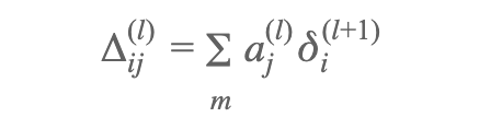
4.3 Perform astern propagation
Then, we have simplified our neural network in figure i to only testify the details to firstly:
- Subtract A1(3) from Y calculate S3
- Thereafter perform a linear equation using the thetas mentioned below multiplied by S3 to calculate. S2.
Since a motion-picture show paints 1000 words, figure ix should explicate what we utilise to calculate S3 and thereafter S2 (marked in cherry).
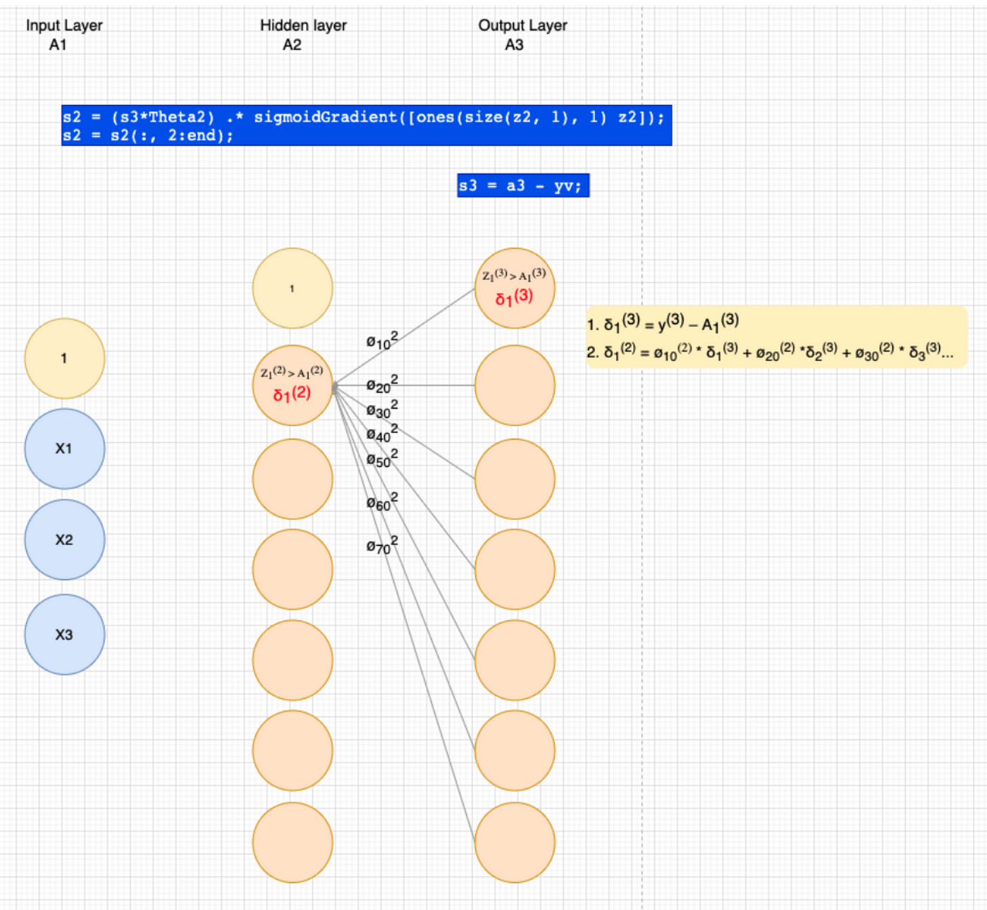
From (3) we sympathise how our weights (thetas) were initialised, so just to visualise the weights (ø) that effigy 9 is referring see figure 10 below.
So once more, with matrix manipulation to the rescue, forward propagation is not a difficult task in python
          # Perform astern propagation to calculate deltas
s3 = a3 - yv
s2 = np.matmul(s3, Theta2) * \
            sigmoidGradient(np.insert(z2, 0, 1, axis=ane))          # remove z2 bias column
s2 = s2[:, i:]
4.4 Summate gradients from backward prop
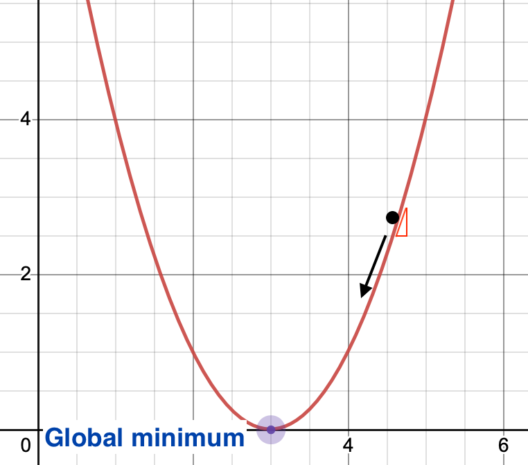
We need to render the gradient's every bit part of our price function, these are needed as gradient descent is a process that occurs in backward prop where the goal is to continuously resample the gradient of the model's parameter in the opposite direction based on the weight w, updating consistently until nosotros reach the global minimum of function J(westward).
To put it only, we use slope descent to minimize the cost function, J(w).
And over again, matrix manipulation to the rescue makes it simply a few lines of lawmaking.
Our start step is to calculate a penalty which tin can be used to regularise our price. If you want an explanation on regularisation, and so accept a await at this article.
          # calculate regularized penalty, replace 1st column with zeros
p1 = (lambda_/one thousand) * np.insert(Theta1[:, 1:], 0, 0, centrality=1)
p2 = (lambda_/yard) * np.insert(Theta2[:, ane:], 0, 0, axis=i)
For cost optimisation, we need to feed dorsum the gradient of this particular fix of weights. Effigy 2 indicates what a gradient is once its been plotted. For the set of weights, existence fed to our cost office, this volition exist the slope of the plotted line.
# gradients / partial derivitives
Theta1_grad = delta_1 / one thousand + p1
Theta2_grad = delta_2 / yard + p2
grad = np.concatenate((Theta1_grad.flatten(),
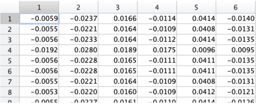
Theta2_grad.flatten()), axis=None) However, the cost optimisation functions dont know how to piece of work with 2 theta'south, so lets unroll these into a vector, with results shown in figure 5.
          grad = np.concatenate((Theta1_grad.flatten(),
            Theta2_grad.flatten()), axis=None)
Ok WOW, thats been a lot of info, but our cost function is done, lets motility onto running gradient descent and cost optimization.
v. Perform cost optimization
5.1 Validating our cost role
I difficult matter to sympathize is if our cost function is performing well. A good method to bank check this is to run a part called checknn.
Creates a small neural network to cheque the backpropagation gradients, it will output the belittling gradients produced by your backprop code and the numerical gradients (computed using computeNumericalGradient). These ii gradient computations should effect in very similar values.
If you lot desire to delve more than into the theory behind this technique, information technology is tought in Andrew Ng's automobile learning course, week iv.
You practise non need to run this every time, only when y'all have setup your cost function for the commencement time.
I won't put the code hither, simply check the github project in checknn.py for the post-obit functions:
- checkNNGradients
- debugInitializeWeights
- computeNumericalGradient
Later on running cheecknn, y'all should get the following results

five.two Slope descent
Slope descent is an optimization algorithm which is mainly used to find the minimum of a office. In machine learning, gradient descent is used to update parameters in a model. Parameters tin can vary according to the algorithms, such as coefficients in Linear Regression and weights in Neural Networks. Nosotros will use SciPy optimize modules to run our gradient descent.
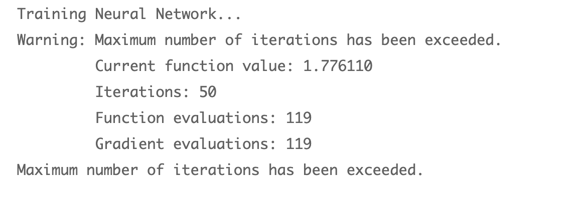
          from scipy import optimize as opt          print('Training Neural Network... ')
#  Modify the MaxIter to a larger value to see how more
#  grooming helps.
options = {'maxiter': 50, 'disp': True}          # You lot should likewise try different values of lambda
lambda_ = i;          # Create cost function shortcuts to be minimized
fun = lambda nn_params: nnCostFunction2(nn_params, input_layer_size, hidden_layer_size, output_layer_size, xn, y, lambda_)[0]          jac = lambda nn_params: nnCostFunction2(nn_params, input_layer_size, hidden_layer_size, output_layer_size, xn, y, lambda_)[1]          # Now, costFunction is a function that takes in only i
# argument (the neural network parameters)          res = opt.minimize(fun, nn_params, method='CG', jac=jac, options=options)          nn_params = res.10
cost = res.fun
impress(res.message)          print(cost)
Get our thetas back for each layer past using a reshape
          # Obtain Theta1 and Theta2 back from nn_params          Theta1 = nn_params[:hidden_layer_size * (input_layer_size +
            one)].reshape((hidden_layer_size, input_layer_size + i))          Theta2 = nn_params[hidden_layer_size * (input_layer_size +
            1):].reshape((output_layer_size, hidden_layer_size + one))
6. Predict results to check accuracy
Now that we have our best weights (thetas), permit's use them to make a prediction to bank check for accuracy.
pred = predict(Theta1, Theta2, Ten) print(f'Training Fix Accurateness: {(pred == y).mean() * 100:f}')
You should become an accuracy of 65.427928%
Yes, it's a trivial low, simply that's the dataset nosotros are working with. I have tried this dataset with logistics regression & SVM and get the same results.
Conclusion
I promise this article gives you lot a deep level of understanding of neural networks and how you can use it to allocate information. Let me know how you go…
Source: https://towardsdatascience.com/the-complete-guide-to-neural-networks-multinomial-classification-4fe88bde7839
0 Response to "Props Cannot Be Imported Again Nureal"
Post a Comment